Agenda

• What makes functions "good"

• Building up functions

• Non-standard evaluation

Learning objectives

• Understand how functions build on top of each other and why "only do one thing" is a good mantra

• Understand non-standard evaluation is, even if you aren't able to fully work with it

What does this mean operationally?

• Your function should do ONE thing (and do it well)

• Careful when naming functions - be as clear as possible

• Embed useful error messages and warnings

  • Particularly if you're working on a package or set of functions or others are using your functions

• Refactor your code to be more clear after initial drafts (it's okay to be messy on a first draft)

Example 1

• Anything we can do to clean this up?

both_na <- function(x, y) {
    if(length(x) != length(y)) {
        lx <- length(x)
        ly <- length(y)
        v_lngths <- paste0("x = ", lx, ", y = ", ly)
        if(lx %% ly == 0 | ly %% lx == 0) {
            warning("Vectors were recycled (", v_lngths, ")")
        }
        else {
            stop("Vectors are of different lengths and are not recyclable:",
                 v_lngths)    
        }
    }
    sum(is.na(x) & is.na(y))
}Copy Code

Calculate if recyclable

recyclable <- function(x, y) {
    test1 <- length(x) %% length(y)
    test2 <- length(y) %% length(x)
    any(c(test1, test2) == 0)
}Copy Code

Test it

a <- c(1, NA, NA, 3, 3, 9, NA)
b <- c(NA, 3, NA, 4, NA, NA, NA)
recyclable(a, b)Copy Code

## [1] TRUECopy Code

recyclable(a, c(b, b))Copy Code

## [1] TRUECopy Code

recyclable(a, c(b, b, b))Copy Code

## [1] TRUECopy Code

recyclable(c(a, a), c(b, b, b))Copy Code

## [1] FALSECopy Code

Revision

both_na <- function(x, y) {
    if(!recyclable(x, y)) {
        stop("Vectors are of different lengths and are not recyclable: ",
             "(x = ", length(x),
             ", y = ", length(y), ")")    
    }
    if(length(x) == length(y)) {
        return(sum(is.na(x) & is.na(y)))
    }
    if(recyclable(x, y)) {
        warning("Vectors were recycled (", 
                "x = ", length(x), 
                ", y = ", length(y), ")")
        return(sum(is.na(x) & is.na(y)))
    }
}Copy Code

Test it

both_na(a, b)Copy Code

## [1] 2Copy Code

both_na(a, c(b, b))Copy Code

## Warning in both_na(a, c(b, b)): Vectors were recycled (x = 7, y = 14)Copy Code

## [1] 4Copy Code

both_na(c(a, b), c(b, b, b))Copy Code

## Error in both_na(c(a, b), c(b, b, b)): Vectors are of different lengths and are not recyclable: (x = 14, y = 21)Copy Code

both_na(c(a, a), b)Copy Code

## Warning in both_na(c(a, a), b): Vectors were recycled (x = 14, y = 7)Copy Code

## [1] 4Copy Code

Anything else?

Make errors/warnings a function

check_lengths <- function(x, y) {
    if(!length(x) == length(y)) {
        if(recyclable(x, y)) {
            warning("Vectors were recycled (", 
                    "x = ", length(x), 
                    ", y = ", length(y), ")")
        }
        else {
            stop("Vectors are of different lengths and are not recyclable: ",
             "(x = ", length(x),
             ", y = ", length(y), ")")
        }
    }
}Copy Code

Revision 2

both_na <- function(x, y) {
    check_lengths(x, y)
    sum(is.na(x) & is.na(y))
}Copy Code

Test it

both_na(a, b)Copy Code

## [1] 2Copy Code

both_na(a, c(b, b))Copy Code

## Warning in check_lengths(x, y): Vectors were recycled (x = 7, y = 14)Copy Code

## [1] 4Copy Code

both_na(c(a, b), c(b, b, b))Copy Code

## Error in check_lengths(x, y): Vectors are of different lengths and are not recyclable: (x = 14, y = 21)Copy Code

both_na(c(a, a), b)Copy Code

## Warning in check_lengths(x, y): Vectors were recycled (x = 14, y = 7)Copy Code

## [1] 4Copy Code

Why would we do this?

• In this case - more readable code

• We might re-use the recyclable or check_lengths functions in other/new functions

• Helps make de-bugging easier

Quick de-bugging example

f <- function(a) g(a)
g <- function(b) h(b)
h <- function(c) i(c)
i <- function(d) {
  if (!is.numeric(d)) {
    stop("`d` must be numeric", call. = FALSE)
  }
  d + 10
}Copy Code

traceback

f("a")
traceback()Copy Code

Note

• Were it not for the tidyverse, I would not even mention NSE

• Generally, it's not an incredibly important topic

• But, NSE is ubiquitous in the tidyverse - literally just about everything uses NSE, which makes programming with tidyverse functions more difficult

What is NSE

• Implementation of different scoping rules

• In dplyr and many others, arguments are evaluated inside the specified data frames, rather than the current or global environment.

How?

(a) Capture an expression (quote it) (b) Use the expression within the correct context (evaluate it)

So, x is evaluated as, e.g., df$x rather than globalenv()$x.

Example

Using the percentile_df function we created previously

• Here base::substitute

percentile_df <- function(x) {
    sorted <- sort(x)
    d <- data.frame(sorted, percentile = ecdf(sorted)(sorted))
    names(d)[1] <- paste0(substitute(x), collapse = "_")
    d
}
percentile_df(rnorm(100, 5, 0.2)) %>%
    head()Copy Code

##   rnorm_100_5_0.2 percentile
## 1        4.384718       0.01
## 2        4.494705       0.02
## 3        4.500262       0.03
## 4        4.562786       0.04
## 5        4.564927       0.05
## 6        4.568238       0.06Copy Code

Confusing

• Outside of a function, substitute operates just like quote - it quotes the input.

• Inside of a function, substitute does as its name implies - it substitutes the input for the name.

Example

quote(subset(df, select = var))Copy Code

## subset(df, select = var)Copy Code

substitute(subset(df, select = var))Copy Code

## subset(df, select = var)Copy Code

extract_var <- function(df, var) {
    substitute(df)
}
extract_var(mtcars)Copy Code

## mtcarsCopy Code

Actually getting this thing to work

extract_var <- function(df, var) {
    subset(eval(substitute(df)), 
           select = var)
}
extract_var(mtcars, "mpg")Copy Code

##                      mpg
## Mazda RX4           21.0
## Mazda RX4 Wag       21.0
## Datsun 710          22.8
## Hornet 4 Drive      21.4
## Hornet Sportabout   18.7
## Valiant             18.1
## Duster 360          14.3
## Merc 240D           24.4
## Merc 230            22.8
## Merc 280            19.2
## Merc 280C           17.8
## Merc 450SE          16.4
## Merc 450SL          17.3
## Merc 450SLC         15.2
## Cadillac Fleetwood  10.4
## Lincoln Continental 10.4
## Chrysler Imperial   14.7
## Fiat 128            32.4
## Honda Civic         30.4
## Toyota Corolla      33.9
## Toyota Corona       21.5
## Dodge Challenger    15.5
## AMC Javelin         15.2
## Camaro Z28          13.3
## Pontiac Firebird    19.2
## Fiat X1-9           27.3
## Porsche 914-2       26.0
## Lotus Europa        30.4
## Ford Pantera L      15.8
## Ferrari Dino        19.7
## Maserati Bora       15.0
## Volvo 142E          21.4Copy Code

Why eval

• substitute is quoting the input, but we then need to evaluate it.

• All of this is rather confusing

• The tidyverse uses it so frequently, they've decided to implement their own version, called tidyeval, which we'll get to in a minute.

Better

Use NSE for both arguments

extract_var <- function(df, var) {
    eval(substitute(var), envir = df)
}
extract_var(mtcars, mpg)Copy Code

##  [1] 21.0 21.0 22.8 21.4 18.7 18.1 14.3 24.4 22.8 19.2 17.8 16.4 17.3 15.2 10.4 10.4 14.7 32.4 30.4 33.9 21.5 15.5 15.2 13.3 19.2 27.3 26.0 30.4 15.8 19.7 15.0 21.4Copy Code

• The above is equivalent to df$var but where both df and var can be swapped programmatically.

• The var argument is being substituted in for whatever the user supplies, and is being evaluated within the df environment

Maybe more simply

extract_var <- function(df, var) {
    df[ ,as.character(substitute(var))]
}
extract_var(mtcars, mpg)Copy Code

##  [1] 21.0 21.0 22.8 21.4 18.7 18.1 14.3 24.4 22.8 19.2 17.8 16.4 17.3 15.2 10.4 10.4 14.7 32.4 30.4 33.9 21.5 15.5 15.2 13.3 19.2 27.3 26.0 30.4 15.8 19.7 15.0 21.4Copy Code

• Why as.character? Otherwise it is a symbol, which won't work.

• Note we could add drop = FALSE to this if we wanted to maintain the data frame structure

Taking this even further

extract_vars <- function(df, ...) {
  vars <- substitute(alist(...))
    df[ ,as.character(vars)[-1]]
}
head(extract_vars(mtcars, mpg, cyl, disp))Copy Code

##                    mpg cyl disp
## Mazda RX4         21.0   6  160
## Mazda RX4 Wag     21.0   6  160
## Datsun 710        22.8   4  108
## Hornet 4 Drive    21.4   6  258
## Hornet Sportabout 18.7   8  360
## Valiant           18.1   6  225Copy Code

• We've now basically replicated dplyr::select

• Notice the use of [-1], because calling as.character on vars always returns alist as the first element in the vector

Why is NSE used so frequently in the tidyverse?

mpg %>% 
  select(manufacturer, model, hwy)Copy Code

## # A tibble: 234 x 3
##    manufacturer model        hwy
##    <chr>        <chr>      <int>
##  1 audi         a4            29
##  2 audi         a4            29
##  3 audi         a4            31
##  4 audi         a4            30
##  5 audi         a4            26
##  6 audi         a4            26
##  7 audi         a4            27
##  8 audi         a4 quattro    26
##  9 audi         a4 quattro    25
## 10 audi         a4 quattro    28
## # … with 224 more rowsCopy Code

Interactive work!

• It makes interactive work easier!

• But this make programming with these functions harder...

• Without NSE, select and similar functions would not know where manufacturer, model, or hwy "live". It would be looking for objects in the global environment with these names.

dplyr programming fail

• Let's say we wanted a function that returned means in a nice table-y format for a variable by two groups (e.g., cross-tab sort of format)

• Typically, we would start by solving this problem for a single situation, then we'd generalize it to a function.

• Let's do it!

mtcars %>%
    group_by(cyl, gear) %>%
    summarize(mean = mean(mpg, na.rm = TRUE)) %>%
    pivot_wider(names_from = cyl, values_from = mean)Copy Code

## # A tibble: 3 x 4
##    gear    `4`   `6`   `8`
##   <dbl>  <dbl> <dbl> <dbl>
## 1     3 21.5   19.75 15.05
## 2     4 26.925 19.75 NA   
## 3     5 28.2   19.7  15.4Copy Code

• Try generalizing the above code into a function

Generalize to a function

Typically, we would expect something like this to work

group_means <- function(data, outcome, group_1, group_2) {
    data %>%
        group_by(group_1, group_2) %>%
        summarize(mean = mean(outcome, na.rm = TRUE)) %>%
        pivot_wider(names_from = group_1, values_from = mean)
}Copy Code

But it doesn't...

group_means(mtcars, mpg, cyl, gear)Copy Code

## Error: Must group by variables found in `.data`.
## * Column `group_1` is not found.
## * Column `group_2` is not found.Copy Code

group_means(diamonds, price, cut, clarity)Copy Code

## Error: Must group by variables found in `.data`.
## * Column `group_1` is not found.
## * Column `group_2` is not found.Copy Code

Why?

• It's looking for an object called group_1 that doesn't exist inside the function or in the global workspace!

The {rlang} version

group_means <- function(data, outcome, group_1, group_2) {
    out <- enquo(outcome) # Quote the inputs
    g1 <- enquo(group_1)
    g2 <- enquo(group_2)
    data %>%
        group_by(!!g1, !!g2) %>% # !! to evaluate (bang-bang)
        summarize(mean = mean(!!out, na.rm = TRUE)) %>%
        pivot_wider(names_from = !!g1, values_from = mean)
}Copy Code

group_means(mtcars, mpg, cyl, gear)Copy Code

## # A tibble: 3 x 4
##    gear    `4`   `6`   `8`
##   <dbl>  <dbl> <dbl> <dbl>
## 1     3 21.5   19.75 15.05
## 2     4 26.925 19.75 NA   
## 3     5 28.2   19.7  15.4Copy Code

group_means(diamonds, price, cut, clarity)Copy Code

## # A tibble: 8 x 6
##   clarity     Fair     Good `Very Good`  Premium    Ideal
##   <ord>      <dbl>    <dbl>       <dbl>    <dbl>    <dbl>
## 1 I1      3703.533 3596.635    4078.226 3947.332 4335.726
## 2 SI2     5173.916 4580.261    4988.688 5545.937 4755.953
## 3 SI1     4208.279 3689.533    3932.391 4455.269 3752.118
## 4 VS2     4174.724 4262.236    4215.760 4550.331 3284.550
## 5 VS1     4165.141 3801.446    3805.353 4485.462 3489.744
## 6 VVS2    3349.768 3079.108    3037.765 3795.123 3250.290
## 7 VVS1    3871.353 2254.774    2459.441 2831.206 2468.129
## 8 IF      1912.333 4098.324    4396.216 3856.143 2272.913Copy Code

Alternative: Pass the dots!

• Note, I've made the function a bit simpler here by removing the spread

group_means2 <- function(data, outcome, ...) {
    out <- enquo(outcome) # Still have to quote the outcome
    data %>%
        group_by(...) %>% 
        summarize(mean = mean(!!out, na.rm = TRUE)) 
}
group_means2(mtcars, mpg, cyl, gear)Copy Code

## # A tibble: 8 x 3
## # Groups:   cyl [3]
##     cyl  gear   mean
##   <dbl> <dbl>  <dbl>
## 1     4     3 21.5  
## 2     4     4 26.925
## 3     4     5 28.2  
## 4     6     3 19.75 
## 5     6     4 19.75 
## 6     6     5 19.7  
## 7     8     3 15.05 
## 8     8     5 15.4Copy Code

group_means2(diamonds, price, cut, clarity)Copy Code

## # A tibble: 40 x 3
## # Groups:   cut [5]
##    cut   clarity     mean
##    <ord> <ord>      <dbl>
##  1 Fair  I1      3703.533
##  2 Fair  SI2     5173.916
##  3 Fair  SI1     4208.279
##  4 Fair  VS2     4174.724
##  5 Fair  VS1     4165.141
##  6 Fair  VVS2    3349.768
##  7 Fair  VVS1    3871.353
##  8 Fair  IF      1912.333
##  9 Good  I1      3596.635
## 10 Good  SI2     4580.261
## # … with 30 more rowsCopy Code

Added benefit

I can now also pass as many columns as I want, and it will still work!

group_means2(diamonds, price, cut, clarity, color)Copy Code

## # A tibble: 276 x 4
## # Groups:   cut, clarity [40]
##    cut   clarity color     mean
##    <ord> <ord>   <ord>    <dbl>
##  1 Fair  I1      D     7383    
##  2 Fair  I1      E     2095.222
##  3 Fair  I1      F     2543.514
##  4 Fair  I1      G     3187.472
##  5 Fair  I1      H     4212.962
##  6 Fair  I1      I     3501    
##  7 Fair  I1      J     5795.043
##  8 Fair  SI2     D     4355.143
##  9 Fair  SI2     E     4172.385
## 10 Fair  SI2     F     4520.112
## # … with 266 more rowsCopy Code

Wait a minute!

• This isn't the same thing

Correct

So in this case passing the dots won't fully fix our problem, but there is another alternative

Alternative syntax

Pipe-centric

• Because the data argument comes first, this function works just like any other in the tidyverse, e.g.,

diamonds %>% 
  filter(color == "E") %>% 
  select(carat, cut, clarity) %>% 
  group_means3(carat, cut, clarity)Copy Code

## # A tibble: 8 x 6
##   clarity       Fair      Good `Very Good`   Premium     Ideal
##   <ord>        <dbl>     <dbl>       <dbl>     <dbl>     <dbl>
## 1 I1       0.9688889 1.330870    1.069545  1.043     1.037778 
## 2 SI2      1.015641  0.8825743   0.9304045 0.9576686 0.8744136
## 3 SI1      0.8670769 0.7238592   0.7230831 0.7262866 0.6706266
## 4 VS2      0.6902381 0.739375    0.6644135 0.6189348 0.5211356
## 5 VS1      0.6328571 0.6806742   0.6097952 0.6431507 0.5035919
## 6 VVS2     0.6007692 0.5601923   0.4267114 0.5115702 0.4839053
## 7 VVS1     0.64      0.4181395   0.4000588 0.4622857 0.4265075
## 8 IF      NA         0.3733333   0.5793023 0.5762963 0.4577215Copy Code

Syntax note

• The {{}} syntax is obviously much easier to apply

• It gets you out of tidyeval complications maybe 80% of the time

• If you start doing a lot of programming w/the tidyverse, you'll probably want to read up more no tidyeval and get comfy with quoting/unquoting

Challenge

• Write a function that summarizes any numeric columns by returning the mean, standard deviation, min, and max values.

• For bonus points, embed a meaningful error message if the columns supplied are not numeric.

Example

summarize_cols(diamonds, depth, table, price)Copy Code

## # A tibble: 3 x 5
##   var         mean          sd   min   max
##   <chr>      <dbl>       <dbl> <dbl> <dbl>
## 1 depth   61.74940    1.432621    43    79
## 2 price 3932.800   3989.440      326 18823
## 3 table   57.45718    2.234491    43    95Copy Code

Pass the dots!

summarize_cols <- function(data, ...) {
    data %>%
        select(...) %>%
        pivot_longer(everything(), 
                     names_to = "var", 
                     values_to = "val") %>%
        group_by(var) %>%
        summarize(mean = mean(val, na.rm = TRUE),
                  sd = sd(val, na.rm = TRUE),
                  min = min(val, na.rm = TRUE),
                  max = max(val, na.rm = TRUE))
}Copy Code

Pipe-centric again

Just putting data as the first argument leads to a lot of benefits

library(palmerpenguins)
penguins %>% 
  select_if(is.numeric) %>% 
  summarize_cols(everything())Copy Code

## # A tibble: 5 x 5
##   var                     mean          sd    min    max
##   <chr>                  <dbl>       <dbl>  <dbl>  <dbl>
## 1 bill_depth_mm       17.15117   1.974793    13.1   21.5
## 2 bill_length_mm      43.92193   5.459584    32.1   59.6
## 3 body_mass_g       4201.754   801.9545    2700   6300  
## 4 flipper_length_mm  200.9152   14.06171    172    231  
## 5 year              2008.029     0.8183559 2007   2009Copy Code

Linearity

• We want to check if an x/y relation is linear

• Function should produce linear and non-linear relations

• Optionally show the data

Maybe this?

check_linear <- function(data, x, y, se = TRUE, 
                         points = FALSE) {
    p <- ggplot(data, aes(x, y)) 
    if(points) {
      p <- p + geom_point(color = "gray80")
    }
  if(se) {
      p <- p +
        geom_smooth(method = "lm") +
        geom_smooth() 
  }
  else {
      p <- p +
        geom_smooth(method = "lm", se = FALSE) +
        geom_smooth(se = FALSE)    
  }
  p
}Copy Code

Nope

check_linear(penguins, bill_length_mm, bill_depth_mm)Copy Code

## Error in FUN(X[[i]], ...): object 'bill_length_mm' not foundCopy Code

Use tidyeval

Note - there are other approaches too, but they are soft deprecated

check_linear <- function(data, x, y, points = FALSE, ...) {
    p <- ggplot(data, aes({{x}}, {{y}})) 
    if (points) {
      p <- p + geom_point(color = "gray80")
    }   
    p + 
      geom_smooth(method = "lm",
                    color = "magenta", 
                      ...) +
      geom_smooth(...)
}Copy Code

check_linear(penguins, bill_length_mm, bill_depth_mm)Copy Code

Add points

check_linear(penguins, bill_length_mm, bill_depth_mm,
             points = TRUE)Copy Code

Add ggplot functions

check_linear(mtcars, disp, mpg, se = FALSE) +
    labs(title = "Checking linearity",
         subtitle = "Linear vs LOESS fits",
         x = "Engine Displacement",
         y = "Miles Per gallon") +
    theme_dark(20)Copy Code

Building up plots

• Let's create a function that calculates means and standard errors for every numeric column in a data frame

• We'll then use this function to create a plotting function

Means/SE's

• First figure it out for a single example

• Note there's not built-in function for the standard error of the mean, which is $\frac{\sigma }{\sqrt{n}}$

# SE function
se <- function(x) {
  x <- x[!is.na(x)]
  sd(x)/sqrt(length(x))
}Copy Code

Full means/SEs

penguins %>% 
  select_if(is.numeric) %>% 
  pivot_longer(everything(),
               names_to = "var",
               values_to = "val") %>% 
  group_by(var) %>% 
  summarize(mean = mean(val, na.rm = TRUE),
            se = se(val))Copy Code

## # A tibble: 5 x 3
##   var                     mean          se
##   <chr>                  <dbl>       <dbl>
## 1 bill_depth_mm       17.15117  0.1067846 
## 2 bill_length_mm      43.92193  0.2952205 
## 3 body_mass_g       4201.754   43.36473   
## 4 flipper_length_mm  200.9152   0.7603704 
## 5 year              2008.029    0.04412279Copy Code

Challenge

Try to generalize the code on the previous slide into a function. Test it on the forcats::gss_cat data.

Translate to a function

estimate_means <- function(df) {
  df %>%
    select_if(is.numeric) %>% 
    pivot_longer(everything(),
                 names_to = "var",
                 values_to = "val") %>% 
    group_by(var) %>% 
    summarize(mean = mean(val, na.rm = TRUE),
              se = se(val)) 
}
estimate_means(forcats::gss_cat)Copy Code

## # A tibble: 3 x 3
##   var            mean         se
##   <chr>         <dbl>      <dbl>
## 1 age       47.18008  0.1181556 
## 2 tvhours    2.980771 0.02429812
## 3 year    2006.502    0.03037436Copy Code

Plot

ggplot(estimate_means(forcats::gss_cat), 
       aes(var, mean)) +
    geom_errorbar(aes(ymin = mean + qnorm(0.025)*se,
                      ymax = mean + qnorm(0.975)*se),
                  width = 0.4,
                  color = "gray40") +
    geom_point() +
    coord_flip()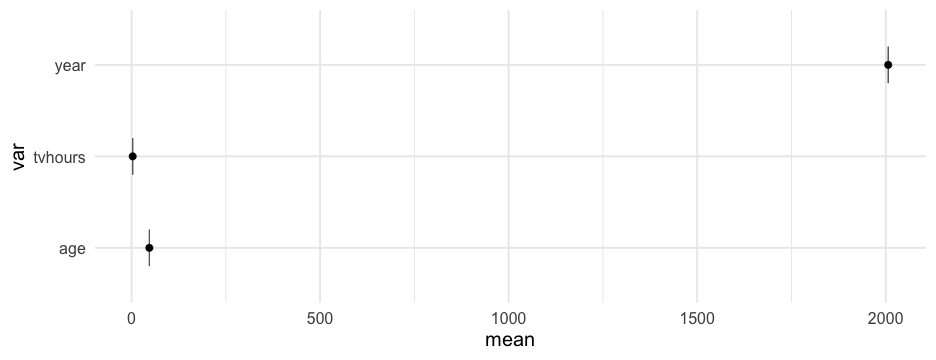Copy Code

Create plot function

plot_means <- function(df) {
  means <- estimate_means(df) %>% 
    mutate(var = reorder(factor(var), mean))
  ggplot(means, aes(var, mean)) +
    geom_errorbar(aes(ymin = mean + qnorm(0.025)*se,
                      ymax = mean + qnorm(0.975)*se),
                  width = 0.4,
                  color = "gray40") +
    geom_point() +
    coord_flip()
}Copy Code

Notice we've successfully avoided tideval entirely in both examples!

Examples

plot_means(penguins)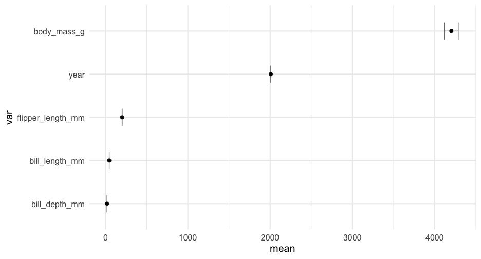Copy Code

plot_means(diamonds)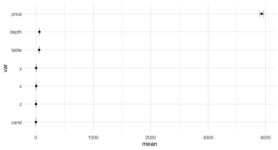Copy Code

Overall takeaway

• Non-standard evaluation is confusing but kind of neat

• Programming with the tidyverse can be a bit more difficult, but not always

• Good to think about multiple ways to approach the same problem (and when programming, perhaps think outside the tidyverse at times)